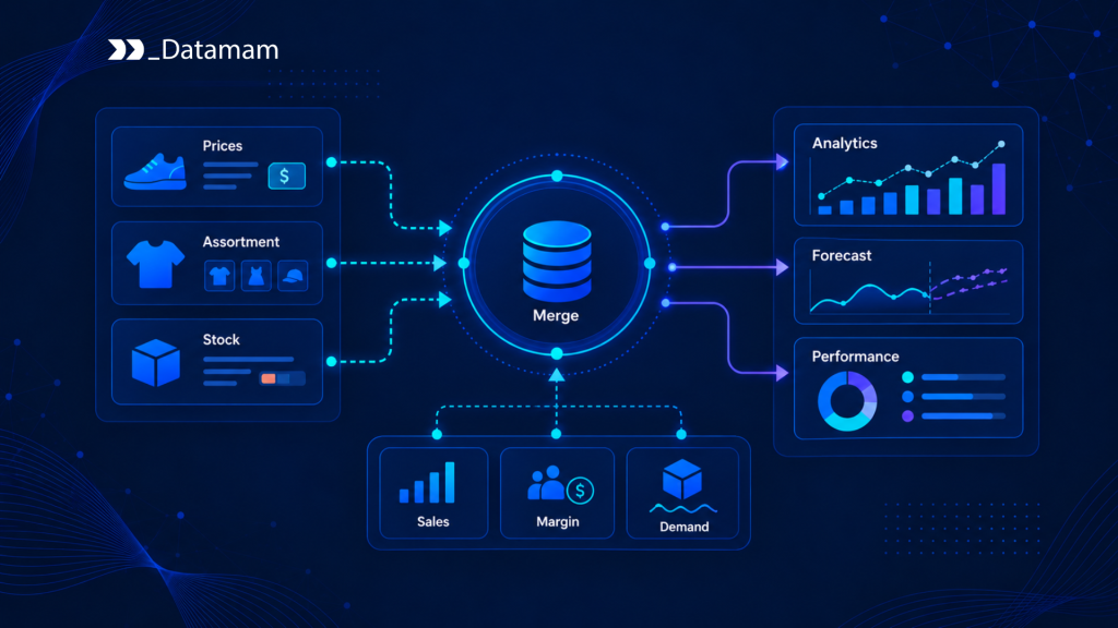
Internal and external retail data rarely arrive in a form that can simply be joined together.
A retailer may record sales at SKU × store × day.
A competitor monitoring system may observe a price at competitor product × selected location × timestamp.
Marketplace data may introduce another level:
product × seller × offer × timestamp.
Assortment data may describe product presence rather than transactions. Stock data may be a point-in-time state. Promotions may apply across intervals rather than individual observations.
All of these datasets can be useful for Retail Analytics, but only if their differences are preserved.
The key problem is therefore not:
How do we put competitor data into the same dashboard as internal data?
It is:
At what product, time, market, channel, and aggregation level are the datasets actually comparable?
A useful Retail Analytics workflow is:
capture → normalize → resolve entities → align analytical grain → align time → align location and channel → handle missingness → aggregate deliberately → join internal data → calculate metrics → interpret
Key Takeaways
- Retail Analytics should align internal and external data at a defined analytical grain before calculating comparative metrics.
- External competitor observations are usually snapshots, while sales, revenue, and margin are often transactions or period aggregates.
- Product matching and category mapping solve different problems and should remain separate.
- A competitor price observed for one store, seller, or delivery market should not automatically be joined to national or unrelated internal performance.
- Missing competitor data can mean source failure, product disappearance, field absence, extraction failure, or simply no scheduled observation. Those states should not collapse into one null value.
- Raw observed fields, normalized fields, derived metrics, and internal business classifications should retain separate lineage.
- When several competitor offers exist for one internal product, the definition of “competitor price” must be explicit.
- External observations can provide market context for retail performance analytics, but they do not by themselves prove why internal sales, margin, or conversion changed.
- Retail analytics software becomes more useful when comparative metrics remain traceable to the source observations and rules that produced them.
Internal and External Retail Data Have Different Structures
Internal retail systems commonly contain data such as:
- transactions;
- daily SKU sales;
- revenue;
- gross margin;
- store inventory;
- promotions;
- returns;
- ecommerce conversion;
- product hierarchy;
- customer or loyalty activity.
External monitoring produces a different type of record:
- competitor product;
- displayed price;
- promotion text;
- observed stock state;
- seller;
- delivery condition;
- selected location;
- listing presence;
- timestamp.
These datasets describe different phenomena.
Internal sales might measure:
142 units sold during Monday.
A competitor record might say:
Product X was observed at $79.99 at 14:05 on Monday for a selected store.
Those records cannot be compared correctly until the analytical relationship between them is defined.
The Deloitte 2026 Global Retail Industry Outlook identifies data-driven insight alongside customer centricity, financial discipline, operational excellence, and adaptability as core retail capabilities. For analytics teams, that makes data semantics important: more sources only help when the resulting metrics remain comparable and interpretable.
Define the Analytical Grain Before Joining Data
The grain of a dataset describes what one row represents.
For example:
| Dataset | Possible Grain |
| Store sales | Internal SKU × store × day |
| Ecommerce sales | Internal SKU × channel × hour |
| Competitor price | Competitor product × retailer × location × timestamp |
| Marketplace offer | Product × seller × marketplace × timestamp |
| Competitor availability | Product × location × timestamp |
| Assortment snapshot | Product entity × retailer × observation period |
| Promotion | Product or group × promotion mechanic × validity interval |
The grain determines which joins are safe.
Suppose an internal table contains:
SKU × store × day
but competitor data contains:
competitor product × retailer × national website × timestamp
Joining the competitor observation to every internal store row can create false local precision.
Likewise, joining ten marketplace seller offers to one internal SKU without aggregation can multiply the internal sales record ten times.
Retail Analytics should therefore establish the target analytical grain before the join.
For example:
internal SKU × market × day
Then each source must be transformed appropriately to that grain.
Product Identity Has to Be Resolved Before Metrics Are Compared
Internal and external product identifiers rarely align automatically.
A retailer might use:
SKU-28471
while a competitor uses:
model_1234_black
and another marketplace identifies offers using a seller-specific listing ID.
Product resolution may use:
- GTIN or UPC;
- manufacturer part number;
- brand;
- model;
- size;
- pack count;
- color;
- configuration;
- category-specific attributes.
The resulting relationship should remain explicit:
- exact product;
- same underlying product, different pack or variant;
- close comparable;
- broader substitute;
- non-comparable;
- unresolved.
This matters because a price-gap metric against an exact product means something different from a price gap against a substitute.
The relationship should travel with the analytical result rather than disappearing after the join.
Product Matching and Category Mapping Are Separate
Product matching asks:
What product is this, and how does it relate to another product?
Category mapping asks:
Where does this product belong in the retailer’s analytical taxonomy?
These can succeed or fail independently.
For example:
- an external product may be confidently identified while its internal category mapping remains ambiguous;
- a product may clearly belong to “Running Shoes” while its exact internal counterpart remains unresolved.
Keeping these processes separate improves:
- exception handling;
- category reporting;
- match-quality measurement;
- taxonomy migrations;
- metric debugging.
A category-level report should not quietly treat uncertain product matches as exact product comparisons simply because category mapping succeeded.
External Snapshots and Internal Events Need Time Alignment
External retail observations are often point-in-time snapshots.
Internal retail data is often event-based or aggregated over a period.
That creates a time-alignment problem.
Suppose competitor prices were collected at:
- 08:00;
- 12:00;
- 16:00;
- 20:00.
Internal sales are summarized by day.
What is the competitor price for that day?
Possible rules include:
- latest observation before transaction time;
- last observation of the day;
- median observed price;
- minimum eligible price;
- time-weighted price where sufficient observations exist;
- promotion interval overlapping the sales period.
Each rule answers a different analytical question.
There is no universally correct daily competitor price.
The calculation should therefore preserve:
- observation timestamp;
- aggregation window;
- maximum acceptable observation age;
- selected aggregation method.
A daily price-position metric should be reproducible from those rules.
Snapshot Data and Period Data Should Not Be Treated as Equivalent
A competitor stock observation such as:
in_stock at 10:30
does not mean:
the competitor was in stock all day.
Likewise:
out_of_stock at 18:00
does not establish when the stockout began.
Retail Analytics should distinguish between:
state observations
- displayed price;
- stock status;
- listing presence;
- seller offer;
- visible promotion state.
and:
period/event metrics
- daily sales;
- weekly revenue;
- promotion-period margin;
- units sold;
- transactions.
When state observations are aggregated into period metrics, the transformation method should be explicit.
Location Scope Must Match the Internal Metric
Competitor pricing and availability can vary by:
- selected store;
- postal code;
- delivery zone;
- region;
- country;
- national ecommerce site.
Internal data may also exist at:
- store;
- region;
- warehouse;
- ecommerce channel;
- national level.
A competitor observation for one selected store should not automatically become the competitor price for every internal store.
Useful external fields can include:
- location_scope;
- store_id where applicable;
- postal code;
- region;
- country;
- delivery zone.
Then the join can determine whether the scopes are compatible.
For example:
competitor selected store in Market A
can potentially join to:
internal stores in Market A
but should not silently populate:
national retail performance.
Channel and Fulfillment Context Also Matter
A marketplace offer, direct retailer website price, pickup price, and delivered offer may represent different commercial conditions.
A useful observation can preserve:
- retailer;
- marketplace;
- seller;
- channel;
- fulfillment mode;
- pickup availability;
- delivery availability;
- delivery charge where observed;
- location scope.
Without those fields, an analytics dashboard may compare:
internal store shelf price
against:
marketplace seller price plus shipping
as though the offers were equivalent.
The issue is not that one offer is invalid.
The issue is that the comparison basis has not been defined.
Raw Observations and Derived Fields Should Remain Separate
A strong Retail Analytics model distinguishes four layers.
Source Observation
What appeared on the source:
- raw product title;
- displayed price;
- promotion text;
- stock message;
- seller name;
- source URL;
- timestamp.
Normalized External Data
What the processing layer resolved:
- product entity;
- normalized unit;
- normalized currency;
- price type;
- promotion mechanic;
- availability state;
- category mapping.
Derived Analytical Metrics
What analytics calculated:
- price gap;
- relative price index;
- assortment overlap;
- competitor availability rate;
- promotion coverage;
- observation age.
Internal Business Enrichment
What comes from retailer strategy:
- key value item status;
- strategic competitor tier;
- category role;
- margin band;
- internal product priority.
These layers should not be flattened into one record without provenance.
For example, a field such as:
competitor_relevance = primary
is not a raw fact collected from the competitor website.
It is internal reference data applied to an observed retailer or seller.
Missing Competitor Data Is Not One Kind of Null
Missing external data can have several meanings.
A price may be absent because:
- the page could not be collected;
- the product was not observed;
- the product page existed but did not display a price;
- the product was unavailable;
- the extraction rule failed;
- the field is not exposed by that retailer;
- no collection was scheduled during the period.
Those conditions should not all produce the same analytical value.
A useful missingness model might distinguish:
- observed;
- field_not_exposed;
- listing_not_observed;
- source_unavailable;
- extraction_failed;
- not_scheduled;
- unresolved.
This is especially important when calculating metrics such as:
competitor price coverage = 72%
Without missingness semantics, the analyst may not know whether the missing 28% represents true catalog absence or collection-quality problems.
Define “Competitor Price” Before Building the Dashboard
One internal product can have many external offers.
For example:
- Competitor A: $98
- Competitor B: $105
- Competitor C: $92
- Marketplace seller 1: $87 + shipping
- Marketplace seller 2: $96
- Competitor D: $89, out of stock
What is the competitor price?
Possible metrics include:
- named competitor price;
- lowest eligible available offer;
- median direct-competitor price;
- median exact-match price;
- availability-adjusted median;
- weighted competitor index;
- price range.
Each provides different information.
Retail data analysis becomes unreliable when dashboards present one number labeled:
competitor price
without defining how it was calculated.
If weighting is used, the weighting rules should also be documented.
For example, internal competitor tiers might determine which retailers contribute to an index.
Price Types Should Remain Distinguishable
The same product page can expose several commercial price states:
- standard price;
- promotional price;
- loyalty price;
- coupon;
- multi-buy;
- marketplace offer;
- cart price;
- unit-normalized price.
These fields should not automatically collapse into one value.
For example:
observed_price = 100
loyalty_price = 85
normalized_unit_price = 8.50
represent different facts.
The analytic layer should decide which value applies to a particular metric.
A base-price index may use one.
A promotion analysis may use another.
A loyalty-market comparison may need both.
Availability Should Affect Specific Metrics, Not Overall Data Validity
An out-of-stock competitor offer can still be valid evidence.
It may remain useful for:
- price history;
- listing history;
- assortment analysis;
- promotion history.
But it may be inappropriate for a metric intended to answer:
What available competitor offers are customers able to buy now?
This suggests metric-specific eligibility.
For example:
eligible_for_price_history = true
eligible_for_assortment_presence = true
eligible_for_available_offer_index = false
The same principle applies when stock status is unknown.
Unknown stock does not make the price observation invalid.
It means some stock-dependent metrics cannot use it safely.
Assortment Metrics Also Need Stable Observation Scope
A competitor moving from 2,000 observed products to 2,300 does not necessarily mean assortment increased 15%.
The apparent change could come from:
- broader crawl coverage;
- restored collection after failures;
- new pagination handling;
- seller duplication;
- changed variant structure;
- regional scope changes.
Before calculating assortment change, Retail Analytics should check:
- observation scope;
- collection completeness;
- product-entity normalization;
- marketplace/seller scope;
- market or location;
- source configuration version.
Only comparable observation periods should be used for longitudinal assortment metrics.
This is the same reason raw page counts are a weak measure of assortment breadth.
External Data Adds Context, Not Automatic Causal Explanation
Combining external and internal data can make performance analysis more informative.
It does not automatically make it causal.
Suppose:
- internal unit sales decline;
- a direct competitor lowers a comparable product price during the same period.
The combined dataset supports a hypothesis:
relative price position may have contributed to the performance change.
It does not establish:
the competitor price caused the sales decline.
Additional evidence may include:
- own promotion history;
- internal availability;
- traffic;
- conversion;
- demand indicators;
- experimentation;
- shopper or transaction evidence.
Retail performance analytics should therefore preserve the distinction between:
observed relationship
and:
causal explanation.
A Retail Analytics Integration Workflow
A functional workflow can be organized as:
capture → normalize → resolve products and entities → map categories → define analytical grain → align time → align location/channel → classify missingness → aggregate external offers → join internal data → calculate metrics → validate → interpret
External Observation Layer
May contain:
- source URL;
- retailer;
- seller;
- raw product;
- displayed price;
- promotion text;
- stock text;
- selected location;
- observed timestamp.
Normalized External Layer
May contain:
- resolved product entity;
- product relationship;
- normalized category;
- normalized price type;
- promotion mechanic;
- availability state;
- normalized location scope;
- data-quality status.
Internal Analytics Layer
May contain:
- internal SKU;
- store/channel;
- units;
- revenue;
- margin;
- inventory;
- internal promotion;
- category role;
- strategic product classification.
Joined Analytical Layer
Should document:
- target grain;
- time-alignment method;
- location relationship;
- external aggregation rule;
- source coverage;
- missingness state;
- rule/model versions.
That makes the resulting metric reproducible.
Validate Join Compatibility Before Calculating Metrics
One useful control is to validate whether an external observation is compatible with the internal metric being calculated.
def evaluate_join_compatibility(internal_row, external_record, policy):
if external_record[“product_relationship”] not in policy[“accepted_relationships”]:
return {“compatible”: False, “reason”: “product_relationship”}
if not policy[“location_is_compatible”](
internal_row[“market_scope”],
external_record[“location_scope”],
):
return {“compatible”: False, “reason”: “location_scope”}
if not policy[“channel_is_compatible”](
internal_row[“channel”],
external_record[“channel”],
):
return {“compatible”: False, “reason”: “channel_scope”}
if external_record[“observation_age”] > policy[“maximum_observation_age”]:
return {“compatible”: False, “reason”: “stale_observation”}
if external_record[“missingness_status”] != “observed”:
return {“compatible”: False, “reason”: “missing_or_unresolved”}
return {
“compatible”: True,
“aggregation_rule”: policy[“external_offer_aggregation”],
}
The example does not use universal numeric thresholds.
The retailer defines compatibility according to:
- analytical use case;
- category;
- market;
- channel;
- observation cadence.
A record that is unsuitable for one metric can still remain valid for another.
Retail Analytics Platforms Should Preserve Metric Definitions
A dashboard should not merely show:
- competitor price index;
- assortment overlap;
- stock advantage;
- promotion intensity.
Each metric should have a definition.
For example:
Competitor Price Index
- Which competitor set?
- Exact matches only or close comparables?
- Available products only?
- Promotional prices included?
- Which currency?
- Which locations?
- What observation window?
- What aggregation rule?
Two analysts can otherwise use the same source data and produce different answers while calling both metrics “competitor price index.”
Metric definitions are part of the analytics model, not documentation added afterward.
The McKinsey analysis of pricing and promotions analytics similarly highlights the value of combining multiple customer, competitor, and company factors rather than evaluating pricing and promotion decisions through isolated metrics. The broader Retail Analytics challenge is to make those inputs comparable before using them together.
How to Measure Integrated Retail Analytics Quality
The number of connected datasets is not a useful success metric by itself.
More useful measures include:
| Area | Example Measure |
| Product resolution | Share of external observations linked to usable product entities |
| Match quality | Precision of reviewed exact/comparable relationships |
| Category mapping | Share correctly mapped to internal analytical taxonomy |
| Grain compatibility | Share of joined records conforming to the target analytical grain |
| Time alignment | Share meeting the metric’s allowed observation window |
| Location alignment | Share mapped to compatible market/location scope |
| Channel alignment | Share with compatible sales and competitor channels |
| Missingness classification | Share of missing external fields with an explicit reason |
| External offer aggregation | Share using documented aggregation logic |
| Price context | Share with usable price type and comparison basis |
| Source coverage | Share of required competitors and markets observed |
| Historical continuity | Share with comparable observation coverage across periods |
| Traceability | Share reproducible from source observations and transformation rules |
These measures test whether the integration itself is trustworthy before analysts interpret the resulting business metrics.
How to Evaluate Retail Analytics Readiness
A retailer combining competitor and internal data should be able to answer:
- What does one row represent in each internal and external dataset?
- What is the target grain of the final analytical table?
- Are product relationships preserved after matching?
- Are product matching and category mapping evaluated separately?
- How are external snapshots aligned with internal transaction or period data?
- What maximum observation age is acceptable for each metric?
- Are store, region, delivery-market, and national observations kept distinct?
- Are direct retail, marketplace, store, and ecommerce channels aligned explicitly?
- Can raw observed fields be distinguished from normalized and calculated values?
- Are internal strategic classifications separated from external observations?
- Does each missing value preserve why the data is missing?
- Can an out-of-stock observation remain valid for price history while being excluded from an available-offer metric?
- When several competitor offers exist, is the aggregation rule documented?
- Are promotional, loyalty, coupon, and standard prices stored separately?
- Are assortment trends calculated only across comparable observation scopes?
- Can analysts trace a dashboard metric back to the source observations and transformation rules that produced it?
- Are analytical relationships presented as evidence rather than automatic causal explanations?
These questions reveal whether a retailer has genuinely integrated competitor intelligence with Retail Analytics or has simply placed two datasets next to each other.
Conclusion
Retail Analytics becomes more useful when internal and external data are joined according to what each dataset actually represents.
Internal transactions, inventory, margin, and conversion often describe events or performance over a period.
Competitor prices, listings, promotions, and stock signals are usually observations of external state at a particular time and market scope.
Before those datasets can support reliable analysis, retailers need to resolve product identity, define analytical grain, align time and location, preserve channel context, classify missingness, and specify how multiple competitor offers are aggregated.
The useful model is not:
collect competitor data → add it to the dashboard
It is:
capture → normalize → resolve → align → aggregate → join → calculate → validate → interpret That structure allows retail performance analytics to add external market context without introducing false precision, duplicated metrics, incompatible comparisons, or causal conclusions that the underlying data cannot support.