
Key Takeaways
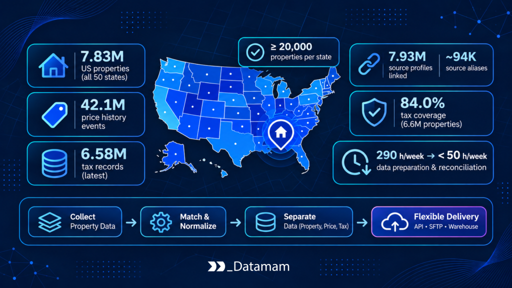
- National Coverage With State Floors: Approximately 7.83 million canonical properties covered all 50 states, enforcing a minimum floor of 20,000 resolved properties per state for regional modeling stability.
- High-Precision Entity Resolution: Property entity matching linked roughly 7.93 million accepted source profiles to the canonical property master while preserving about 94,000 additional source aliases in a dedicated mapping ledger.
- Auditable Event Separation: The curated history table retained over 42.1 million price events across roughly 6.27 million properties, while duplicate observations (7.49 million) and quarantined rows (686,000) were tracked in separate audit ledgers.
- Validated Tax Coverage: Latest tax observations covered nearly 6.6 million properties (84.0% of the release), explicitly separating assessment values from annual tax charges.
- Operational Efficiency: Replacing fragmented regional spreadsheets with a normalized multi-grain warehouse schema reduced analyst data preparation and manual reconciliation from roughly 290 staff hours per week to under 50 hours per week.
Building a national valuation or market-intelligence model requires more than extracting active real estate listings. When an enterprise property analytics business approached Datamam to build a US address foundation connected to physical property attributes, multi-year price history, and the latest available tax assessments, the core challenge was structural fidelity. In a comprehensive real estate data case study, the technical difficulty rarely lies in fetching a single property web page; it lies in preventing historical listing events, tax assessments, and multiple source URLs from corrupting the underlying property count.
To establish the required fields and event structures, our engineering team executed an initial three-ZIP schema assessment before scaling to a national acquisition scope of five to eight million address records across all 50 states. Over a 21-day main collection window and a 48-hour bounded recovery period, Datamam operated a national property portal collection and normalization pipeline that resolved 7,832,636 canonical properties, 42,124,538 accepted price-history events, and 6,577,944 latest tax observations.
By delivering a normalized Snowflake data model that strictly separated physical properties, source profiles, and dated historical events, the architecture allowed downstream analysts to count distinct residential units accurately, evaluate price trajectories at the event grain, and trace every published metric back to its raw capture evidence.
The Problem With One Row for Everything
At the outset of the engagement, the requested field list appeared straightforward: street address, bedroom and bathroom counts, square footage, current market status, text description, home type, all available price-history rows, and the latest tax-history entry. In practice, flattening these attributes into a single wide table creates severe analytical distortion.
A physical residential property frequently accumulates multiple source URLs over time, undergoes multiple listing episodes across different brokerages, and generates dozens of historical price adjustments. Furthermore, a property’s current asking price, its prior closed sale price, an automated valuation model (AVM) estimate, and its county tax assessment represent fundamentally different financial concepts measured at different timestamps. Combining those figures into a single flattened row makes it easy to overwrite prior transaction history, double-count homes during geographic aggregations, or misinterpret a rental asking price as a fee-simple sale.
Prior to this pipeline, the client’s baseline workflow relied on collecting regional file subsets and reconciling separate exports manually. Across a four-week baseline audit, address standardization, duplicate review, history reshaping, and cross-file reconciliation consumed roughly 290 staff hours per week.
To eliminate that bottleneck and separate property records from listing events, the national acquisition enforced a strict relational contract across three distinct data grains:
1. Property Master Record: Represents a single resolved physical property or distinct residential unit.
2. Source-Profile Record: Represents a collected source identity (platform profile URL or identifier) at observation time.
3. History Event Record: Represents an accepted, dated historical event with its original source label, currency, and price basis retained.
Establishing that separation prior to acquisition dictated how the discovery queues, acceptance checks, Snowflake delivery tables, and downstream aggregation rules operated.
Discovering Properties Through Geographic Queues
Before launching national discovery, Datamam engineered a three-ZIP metropolitan pilot fixture in Colorado to exercise dense condominium buildings, side-by-side duplexes with fractional street numbers, detached single-family homes, and modern multi-unit infill developments.
Two specific regression cases from that pilot shaped the production schema:
Multi-Unit Base Address Disambiguation: One regression case paired a building-level profile with two separately identified residential units sharing the exact same base street address.
Fractional House Numbers: Another regression case preserved a primary house number ending in 1/2 (for example, 124 1/2 Main St), which naive integer parsers routinely truncate or corrupt.
Resolving these edge cases established separate building and unit identities alongside a lossless string-based house-number field before national discovery began.
During national execution, geographic discovery accumulated approximately 8.41 million candidate URL references. URL canonicalization—normalizing structural parameters and resolving equivalent references—removed roughly 303,000 repeated or equivalent links, leaving 8,103,324 distinct profile jobs. State-level queues, browse-segment checkpoints, and template-specific adapters organized that workload.
Every queued job retained its discovery state, ZIP context, browse parent, available source identifier, and first-seen timestamp. When a portal issued HTTP redirects or modified URL paths over time, the pipeline appended the new source-reference evidence to the same discovery trail rather than creating an unlinked duplicate record.
Crucially, discovery context and property geography remained separate fields. A property page discovered through one browse area could report a physical street address inside an adjacent jurisdiction. Final coverage reporting used the accepted property’s normalized state, while the original browse context remained available for investigating boundary discrepancies. Segment checkpoints recorded completed, pending, and interrupted discovery slices so that re-running a segment resumed unfinished work cleanly and reused existing identities for rediscovered URLs.
Turning Geographic Balance Into a Coverage Rule
Because the business rationale was regional valuation-model development, each state required a statistically usable foundation for feature engineering and benchmarking. Unconstrained property crawls naturally over-index on high-turnover sunbelt markets while leaving smaller states under-represented. To guarantee national balance, Datamam enforced a floor of 20,000 resolved properties per state, then allocated the remaining collection capacity across approved geographic priorities and eligible source supply.
High-population states such as Texas, California, and Florida received larger proportional collections, while the 20,000-property floor reserved explicit coverage for smaller states such as Wyoming and Vermont. Importantly, state coverage was counted *after* entity resolution: each canonical property contributed once to its state total, while unresolved addresses and failed profiles remained isolated in the exception workflow.
| State Coverage Group | Accepted Canonical Properties | Share of National Release |
| Texas | 718,493 | 9.17% |
| California | 642,817 | 8.21% |
| Florida | 593,284 | 7.57% |
| New York | 411,976 | 5.26% |
| Pennsylvania | 334,718 | 4.27% |
| Vermont | 27,849 | 0.36% |
| Wyoming | 24,613 | 0.31% |
| Remaining 43 States | 5,078,886 | 64.84% |
| Total Across 50 States | 7,832,636 | 100.00% |
The release specification recorded all 50 individual state counts and the effective discovery scope so analysts could account for intentional geographic quotas when building regional valuation models or assessing coverage bias.
Additionally, the schema separated postal delivery codes from statistical spatial areas. Postal ZIP codes remained source address components, whereas geographic analysis stored Census ZIP Code Tabulation Area (ZCTA) identifiers in a separate column. As the U.S. Census Bureau’s guidance on ZIP Code Tabulation Areas explains, postal ZIP codes represent linear mail delivery routes rather than stable geographic polygons; maintaining ZCTAs in a separate field allows analysts to distinguish statistical areas from postal addresses accurately.
Normalizing Addresses Without Erasing Units
Robust real estate address normalization must support deterministic entity matching without erasing the raw evidence needed for auditing. The address model retained the original source string alongside parsed fields for street number, street name, pre- and post-directional components, street suffix, secondary unit designator, unit value, city, state, and ZIP code. All ZIP codes were stored as strings (VARCHAR) so leading zeros in northeastern states survived file export and cloud warehouse loading intact.
Secondary-unit handling followed the official distinctions in USPS Publication 28 (Postal Addressing Standards), including apartment (APT), suite (STE), floor (FL), and unit (UNIT) designators. Normalization preserved the original unit value even when the designator was standardized to a canonical USPS abbreviation. Consequently, Apartment 2 and Apartment 12 received distinct unit identities while connecting back to their shared physical structure through an explicit building-to-unit relationship. Profiles with missing unit details entered identity review whenever structural or spatial evidence indicated a multi-unit property.
The house-number parser preserved alphanumeric suffixes, fractional numbers (1/2), directional prefixes, and hyphenated forms. Address syntax checks and mail-deliverability verification occupied separate fields and validation states, while storing original strings and normalization rule versions ensured that every address decision remained reproducible from retained evidence.
Resolving Source Profiles to Property Identity
Across the national run, acquisition accepted 7,926,202 source profiles. Property entity matching assigned 93,566 additional profiles to properties already represented in the property master, yielding 7,832,636 canonical properties.
Rather than relying on single-field string similarity, matching combined five hierarchical signals:
1. Native source identifiers.
2. Explicit redirect chains captured during discovery.
3. Normalized street and secondary-unit address components.
4. Unit-level structural evidence.
5. Geographic coordinates.
Coordinates narrowed candidate blocking sets, while unit-level identifiers and normalized address evidence determined the final relationship.
# Illustrative Python logic demonstrating multi-grain entity resolution key generation
from dataclasses import dataclass
from typing import Optional
import hashlib

@dataclass(frozen=True)
class NormalizedAddress:
    state: str
    zip5: str
    street_num_raw: str      # Preserves fractional/hyphenated forms like '124 1/2'
    street_pre_dir: str
    street_name: str
    street_suffix: str
    unit_designator: Optional[str]  # USPS Pub 28 standard (e.g., 'APT', 'UNIT')
    unit_value: Optional[str]

def build_property_resolution_keys(addr: NormalizedAddress) -> dict:
    """
    Generates separate deterministic hashes for the base structure and the specific unit
    so multi-unit buildings are never collapsed into a single property row.
    """
    base_tokens = "|".join([
        addr.state.strip().upper(),
        addr.zip5.zfill(5),
        addr.street_num_raw.strip().upper(),
        addr.street_pre_dir.strip().upper(),
        addr.street_name.strip().upper(),
        addr.street_suffix.strip().upper(),
    ])
    building_key = hashlib.sha256(base_tokens.encode("utf-8")).hexdigest()

    if addr.unit_value:
        unit_tokens = f"{base_tokens}|{addr.unit_designator or 'UNIT'}|{addr.unit_value.strip().upper()}"
        canonical_key = hashlib.sha256(unit_tokens.encode("utf-8")).hexdigest()
        grain = "RESIDENTIAL_UNIT"
    else:
        canonical_key = building_key
        grain = "STRUCTURE_OR_PARCEL"

    return {
        "building_key": building_key,
        "canonical_property_key": canonical_key,
        "identity_grain": grain
    }
A separate alias mapping table linked historical source references to each canonical property, while building-to-unit relationships used their own dedicated relationship type. This design kept source identities, physical structures, and residential units independently queryable. Ambiguous relationships retained distinct source-scoped identities flagged with a review status, and accepted merges recorded their supporting evidence and rule version. In a post-processing QA audit, only 15 of 10,000 sampled identity decisions required correction—a 99.85% sample agreement rate across unit-level matches, redirects, and address variants.
Extracting the Entire Visible Price History
In large-scale property history data collection, a property page that loads with a valid HTTP status can still contain an incomplete or unexpanded history section. Collection adapters verified the returned history structure and any pagination or continuation state before marking a profile’s history section complete.
Across the project, the raw history ledger accumulated about 50.3 million history-row observations, which validation partitioned into three explicit categories:
Curated Accepted Events (42,124,538 rows): Validated, deduplicated historical price events published to the analytical warehouse table.
Repeated Evidence (7.49 million rows): Duplicate observations across alias profiles or repeat checks, preserved in a separate occurrence ledger.
Quarantined Observations (686,000 rows): Observations withheld due to unresolved dates, ambiguous amount units, or unmapped event classifications, with exact category counts retained in the supporting exception ledger.
Events with an undisclosed transaction amount remained valid whenever their property link, date, and event classification met acceptance rules; in those cases, the amount field stayed NULL rather than defaulting to zero.
Deduplication used native source event identifiers where available and versioned row fingerprints otherwise. Distinct market actions sharing the same calendar date retained separate event identities, while the occurrence ledger preserved repeated evidence and original source labels. When a source correction occurred on a subsequent check, the pipeline created a versioned revision with the earlier date, label, and amount preserved in the audit trail. Accepted price history covered roughly 6.27 million properties (80.1% of the release), with explicit section statuses distinguishing confirmed empty histories, pending sections, and quarantined observations for the remaining homes.
Separating Asking Prices, Reported Sales, and Estimates
To build a US property dataset with price history that quantitative researchers can trust, the data model must strictly separate asking prices, closed transaction prices, and algorithmic estimates. Each accepted event retained its source label, event date, observed amount, currency, amount basis, source profile link, and capture timestamp. Date-only source values used a strict DATE type, preserving the exact precision supplied by the source without inventing time-of-day components.
The normalized event taxonomy distinguished listing originations, price reductions, listing removals, rental offerings, and reported sales:
Rental amounts carried an explicit rental basis and billing period.
Sale and listing amounts carried a purchase-price or asking-price basis.
Valuation estimates occupied an independently identified measure field.
Whether teams are working with public county records, MLS feeds, or evaluating Zillow property data benchmarks, distinguishing transaction history from automated valuation models is essential. For example, as documented in Zillow’s explanation of the Zestimate, an automated valuation is an estimated market value rather than an official appraisal or verified sale price, and portal price histories frequently combine MLS feeds with county records via third-party aggregators. Retaining the source context, event date, and first-observed timestamp allowed analysts to trace every record to its exact collection window.
Similarly, derived historical price-per-square-foot calculations required an area observation appropriate for the event period. Whenever a property underwent an extension or renovation that altered living area, the schema required a corresponding area version before publishing a historical per-square-foot ratio.
Retaining the Latest Tax Row With Its Reporting Year
To normalize property tax and assessment history, the dedicated tax table held the latest accepted observation for 6,577,944 properties—covering 84.0% of the national release—while explicit availability and validation statuses accounted for the remaining 16.0%.
Because public portals frequently display tax billing years alongside older municipal assessment years, the tax schema separated five core attributes:
1. Tax billing year.
2. Assessment year (when explicitly supplied).
3. Annual tax amount billed.
4. Assessed taxable value.
5. Observation capture timestamp.
An ambiguous source year retained its original label and entered a review state. Assessment amounts and annual tax charges remained distinct measures: a missing component stayed NULL, whereas a valid disclosed zero retained its source context. Year-over-year percentage changes were calculated only between compatible measures and sequential reporting years.
For canonical properties linked to multiple accepted source profiles, a deterministic selection rule recorded the chosen tax observation and its supporting evidence while preserving conflicting values in separate provenance states. If an official county assessor document or tax bill is integrated later, it attaches as an additional verified evidence record without overwriting the original portal observation.
Checking Attributes and Source Status Independently
Physical property attributes—bedrooms, bathrooms, living area, lot size, home type, description, and market status—were validated independently. Optional attributes used nullable columns, and each field retained its own validation status so a missing or malformed secondary attribute never forced the rejection of a valid property record.
Strict data typing prevented silent precision loss across analytical queries:
Bathrooms: Typed as DECIMAL(4,2), preserving quarter-bath values such as 1.75 exactly.
Living and Lot Area: Occupied separate columns, retaining raw source units (sqft, acres) alongside normalized numeric values. When a source profile disclosed a living-area range on new construction, the parser populated explicit min_sqft and max_sqft columns.
Market vs. Retrieval Status: Property status captured both the raw source wording and its normalized category at observation time (for sale, for rent, sold, or off market). Crucially, HTTP retrieval health used a separate collection-status field, keeping a transient network or access error distinct from a real-world market-status change.
Property capture timestamps, historical event dates, and tax reporting years remained independent dimensions so analysts could inspect the observation window, market-event period, and tax period directly. In a QA audit of 12,500 sampled history records, only 65 discrepancies occurred across event dates, labels, amount bases, and property assignments—achieving 99.48% sample agreement.
Completing Acquisition Under a Bounded Recovery Policy
To maintain predictable throughput across millions of pages, discovery, retrieval, history parsing, identity review, and warehouse delivery operated across separate asynchronous queues.
During parsing, template adapters first inspected structured JSON state embedded within initial HTML responses and used secondary data requests only when dynamic history sections required additional hydration. Both paths recorded the template version and section-completeness evidence. Whenever requests encountered rate limits or access challenges (HTTP 403 or HTTP 429), jobs entered explicit collection states. The orchestrator managed egress pool rotation, maintained session consistency, and rescheduled eligible jobs using bounded exponential backoff with jitter while preserving strict retry budgets. Waiting requests immediately released their worker slots, and parser recovery replayed retained raw payloads from staging storage without re-requesting pages over the network.
The production retrieval fleet comprised 16 asynchronous processes with 12 application-request slots each (192 total concurrency slots). Across its busiest five-minute interval, the fleet averaged 42.6 attempts per second, while the once-per-second in-flight gauge reached 86 concurrent requests with a 1.48-second mean request occupancy.
At the conclusion of the 21-day main collection window and 48-hour recovery period, approximately 8.10 million admitted profile jobs reconciled cleanly:
| Acquisition Outcome | Profile Jobs | Share of Admitted Jobs |
| Accepted Source Profiles | 7,926,202 | 97.81% |
| Completed Pages Outside Property-Profile Contract | 64,854 | 0.80% |
| Unresolved at Recovery Cutoff | 112,268 | 1.39% |
| Total Admitted Profile Jobs | 8,103,324 | 100.00% |
Valid terminal outcomes covered 98.61% of admitted jobs, with accepted residential property profiles representing 97.81%. Completed pages outside the residential property contract (such as neighborhood directories or commercial listings) received their own outcome category, while the 112,268 unresolved jobs were delivered in the exception ledger with their final status, attempt history, and discovery context preserved.
Measuring Transfer and the Published Data Objects
Across the 23 elapsed days, the acquisition and recovery workload executed roughly 18.6 million initial document and data requests plus 605,000 retry attempts—totaling 19.2 million attempts and 2.87 TB of application response bodies (accounting for request uploads, protocol overhead, static assets, and rendering separately). Across the full run, throughput averaged 9.7 attempts per second and 124.7 GB of response-body transfer per day (~11.5 Mbps), governed by per-source rate limits and queue budgets.
Temporary raw storage peaked at approximately 242 GB of compressed response payloads at the recovery cutoff. To control storage costs while supporting parser replay during the run, the staging Amazon S3 bucket enforced a seven-day lifecycle expiration rule on raw-response objects. As explained in the AWS documentation on Amazon S3 Object Lifecycle Management, S3 evaluates lifecycle rules once daily and removes expired objects asynchronously, meaning physical bucket size trailed the strict seven-day window slightly even though billing stops upon expiration. Delivery manifests, curated datasets, and operational logs used separate buckets and retention policies.
The full-scope delivery specification published 56,535,118 curated rows across three primary analytical tables:
| Core Delivery Dataset | Curated Rows | Delivery Format |
| Canonical Properties (Property Master) | 7,832,636 | Snappy Parquet |
| Accepted Price Events (Price History) | 42,124,538 | Snappy Parquet |
| Latest Tax Observations (Tax History) | 6,577,944 | Snappy Parquet |
| Total Across Three Core Tables | 56,535,118 | Snappy Parquet |
In production, the Snappy-compressed Apache Parquet batches totaled 14.2 GB in Amazon S3 (partitioned by canonical property state) and occupied 11.8 GB of active table storage inside Snowflake, while source profiles, identity mappings, job ledgers, and exceptions resided in supporting warehouse tables.
Publishing Tables That Preserve Their Grain
The delivery pipeline published Snappy-compressed Parquet batches through Amazon S3 and loaded them into Snowflake staging tables using COPY INTO statements after running automated field validation and referential integrity checks. In accordance with Snowflake’s micro-partition and data loading architecture, Snowflake automatically organized the ingested columnar batches into compressed micro-partitions optimized for analytical query pruning.
Accompanying manifest files recorded the dataset version, acquisition cohort, schema version, object checksums, row counts, and source-observation intervals. Publication reconciled six distinct tables independently: the canonical property master (~7.83M rows), source property profiles (~7.93M rows), property-profile identity mappings, price-history events (~42.12M rows), latest tax observations (~6.58M rows), and collection job audit records (~8.10M rows).
To prevent accidental fan-out joins when analysts combined property attributes with multi-row price histories, consumer views exposed distinct-property counts and event counts as separate semantic measures, aggregating geographic property summaries at the canonical-property grain *before* joining event-level metrics. Delivery replay relied on batch identifiers and record version numbers to guarantee idempotency, while strict referential checks required every accepted price event and tax row to link to an accepted canonical property.
What Changed for the Analytics Team
The normalized Snowflake release connected roughly 7.83 million canonical properties to their source identities, over 42.1 million accepted price events, and nearly 6.6 million latest tax observations—with reconciled counts for coverage, history availability, and collection exceptions.
Instead of reshaping nested JSON arrays or reconciling conflicting regional spreadsheets by hand, analysts could filter price events directly by transaction basis, compare tax billing years against assessment years, and trace 94,000 profile aliases to their canonical residential units.
Across four-week pre- and post-pipeline audits, weekly analyst hours spent on address preparation, duplicate review, history reshaping, and reconciliation dropped from about 290 hours per week to under 50 hours per week—a reduction of roughly 240 hours weekly (83% of manual preparation effort). Because engineering, collection operations, ongoing maintenance, and cloud compute belong to separate cost accounts, leadership could evaluate those operational investments directly against the 240-hour weekly analyst time savings. Most importantly, the modeling team gained an auditable national property foundation ready for feature engineering, coverage analysis, and out-of-time transaction validation.
Frequently Asked Questions
Did every collected source profile become a separate property?
No. Roughly 7.93 million accepted source profiles resolved to 7,832,636 canonical properties. A separate alias mapping table retained 93,566 additional source references alongside their deterministic matching evidence.
Was history available for every property?
No. Accepted price history covered roughly 6.27 million properties (80.1% of the canonical release), and latest tax observations covered nearly 6.58 million properties (84.0%). Empty, pending, and withheld sections retained distinct availability status codes so analysts could distinguish confirmed zero-history homes from validation exceptions.
Did geographic balance mean identical state counts?
No. Regional valuation-model coverage motivated a floor of 20,000 resolved canonical properties per state (ensuring baseline coverage in smaller states like Wyoming and Vermont). Approved geographic priorities and eligible source coverage determined the remaining allocation, resulting in larger collections in Texas, California, and Florida while retaining all 50 state totals in the release specification.
If your organization needs to acquire, deduplicate, and structure multi-million-record property datasets without flattening historical events, explore Datamam’s data normalization services to discuss your geographic scope, property identity rules, and cloud warehouse delivery requirements.
