
Key Takeaways
- Fixed broadband availability and mobile modeled coverage require separate calculations and should never be placed in one unqualified coverage percentage.
- Compare providers using a common reporting date, technology definition, geography, and service threshold.
- Coverage overlap at an address is not the same as active subscriptions, market share, or measured quality.
- Population-weighted and business-weighted measures may answer different commercial questions than area coverage.
- Treat missing records, source revisions, and genuinely unavailable service as different states.
- Report confidence and source limitations alongside every competitive coverage score.
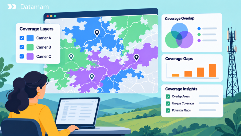
Telecom coverage analysis compares where competing networks can actually offer a service under consistent geographic, technical, and reporting assumptions. It is central to market entry, retention strategy, regulatory research, and infrastructure investment. Yet the word coverage can refer to a serviceable fixed-broadband address, a modeled mobile radio footprint, an observed connection, or simply the number of people living inside a polygon. Those measurements answer different questions.
A useful study therefore defines its unit of analysis before calculating any percentages. For a regional ISP, the key unit may be broadband-serviceable locations that have two or more facilities-based alternatives. For a mobile operator, it may be residents or business sites inside comparable outdoor model polygons. This guide shows how to combine coverage evidence without converting uncertainty into false precision.
What Does Telecom Coverage Analysis Measure?
Coverage analysis measures the footprint of a defined service under an explicit definition of availability. It can answer how many eligible locations an operator reports serving, what share of residents falls within a modeled mobile footprint, or where competing offers overlap. Start with an observation unit, a technology filter, a reference date, and an evidence source; otherwise a convincing map may still produce the wrong business interpretation.
Geographic reach, address-level availability, and population exposure
Geographic reach is usually an area measure, expressed in square kilometers or share of a defined boundary. Address-level availability is a count or proportion of locations that can receive qualifying service, commonly using location identifiers in the FCC’s National Broadband Map. Population exposure overlays coverage with population geography to estimate how many people reside inside the claimed footprint. A carrier can cover a large rural area yet reach fewer residents than a competitor with a compact metropolitan footprint. Each measure needs a denominator: total territory, eligible locations, or estimated population. Report the unit beside the result, not in a footnote that readers can overlook.
Coverage versus network quality and customer adoption
Reported availability identifies potential access, not the quality of the connection delivered at each eligible location. Measured throughput, latency, and reliability require their own testing program; active adoption requires subscriptions or credible customer estimates. One operator may show widespread 5G coverage while another has better measured consistency in congested neighborhoods. Similarly, a provider reporting fiber to thousands of locations may have a low take rate. Competitive assessments should present availability, observed experience, and adoption as separate layers that can later be analyzed together. Blending them into a single ‘network strength’ score without clear weights makes comparisons difficult to audit.
Which Data Sources Are Suitable for Coverage Comparison?
Source selection should follow the commercial question and the required spatial precision. A national planning screen may accept aggregated public data, whereas an address-level overbuild decision needs provider-specific records and a verified location universe. Record each source’s publisher, vintage, spatial resolution, licensing conditions, and whether it reflects a regulatory filing, a consumer offer, or an actual measurement.
Fixed broadband availability records
In the United States, the FCC’s Broadband Data Collection provides provider-reported fixed broadband availability using broadband-serviceable locations and technology and advertised-speed attributes. Data can be explored interactively and downloaded in CSV form through the FCC’s map download guidance. The underlying Fabric is separately licensed, so public availability exports should not be mistaken for unrestricted access to every Fabric field. Use a consistent publication vintage and identify changes in the location universe before calculating growth. An appearing record can reflect a correction, a new location, or service expansion; a temporal comparison needs to distinguish those cases.
Mobile coverage models and network measurements
Mobile availability datasets typically describe modeled propagation under predefined outdoor or in-vehicle assumptions. The FCC explains that the resulting areas are not guarantees of indoor coverage or of identical performance across devices, terrain, and congestion. Independent speed tests and drive-test programs can challenge or enrich a model, but they reflect sampled usage and different technical conditions. The Opensignal measurement approach, for example, distinguishes real-world network experience from a coverage claim. Overlay models and measurements when the data rights permit, but retain source type and confidence. Do not redraw a carrier’s entire footprint from a handful of successful tests.
Independent geographic reference datasets
Population grids, Census geographic boundaries, residential building inventories, and business-establishment data supply denominators for coverage metrics. The US Census Bureau’s internet-use resources can also add adoption context, although household estimates are not address-level provider observations. When aggregating coverage polygons to tracts or counties, avoid treating population as uniformly distributed across a large area. Use appropriate spatial intersections, disclose boundary vintage, and account for uninhabited land. A business-focused operator may deliberately weight workplaces, industrial parcels, or commercial addresses more heavily than residential population, provided those weights are stated.
How to Measure Coverage Overlap Between Providers
Overlap is meaningful only when each provider is evaluated under the same service definition. Choose the common location or polygon universe, normalize legal operators and retail brands, filter technologies and speed thresholds, and then calculate which observations have one, two, or several qualifying facilities-based competitors. Preserve the raw records so alternative thresholds can be rerun.
Comparing serviceable-location records
For fixed broadband, begin with a common set of location IDs and a chosen reporting vintage. Group availability rows by location, facilities-based provider, and technology; deduplicate multiple speed tiers from the same operator before counting competitors. A location with two fiber providers and one cable provider may be classified differently from one with three retail brands using one access network. Produce counts such as ‘locations with at least two fiber competitors’ and ‘locations with no reported terrestrial service meeting the defined threshold.’ Avoid interpreting an unmatched address as unserved. Retain source version, missing-state flags, and changed Fabric IDs so year-over-year comparisons are reproducible.
Overlaying mobile coverage polygons
For mobile providers, standardize the coordinate reference system, technology category, and minimum modeled speed before intersecting polygons. Calculate overlap as a share of the chosen study area and, where useful, as the share of an independently sourced population grid falling within overlapping footprints. Geometry repair may be necessary if polygons contain gaps, invalid rings, or multipart shapes. Very fine overlays can imply precision that the radio models cannot substantiate. Publish a map scale consistent with model resolution and avoid deriving indoor availability, signal strength, or capacity from the mere fact that two polygons overlap.
Weighting coverage by population and business locations
A weighted comparison asks who or what is exposed to a provider’s reported footprint rather than how much empty land it covers. For population exposure, intersect standardized coverage geometries with census geography and calculate an estimated covered population under a disclosed allocation method. For a business-connectivity use case, weight verified establishments or priority premises. Also, for example, covering 80 percent of territory and 40 percent of target business sites is different from covering 35 percent of territory and 90 percent of those sites. Neither measure is universally better; the correct denominator depends on the decision. Quantify sensitivity to grid size, uncertain geocoding, and boundary definitions.
Identifying Geographic Coverage Gaps
A gap can mean no qualifying reported providers, only one credible alternative, weak observed performance, or an excluded technology class. Choose the definition before ranking locations. Geographic absence in a database is also not proof of service absence; it may indicate incomplete source coverage, delayed updates, or unresolved location matching.
Single-provider and multi-provider locations
Classify broadband-serviceable locations by the number of distinct qualifying providers under one common threshold. Zero-provider locations may warrant validation for service gaps; single-provider locations may be candidates for competition analysis; locations with multiple providers require differentiation rather than the assumption of a universal price war. Provider counts should distinguish facilities-based networks from resale brands. A county average can conceal blocks with no competition beside dense clusters of alternatives, so summarize counts at the smallest reliable unit and only then aggregate to market boundaries relevant to the operator.
Areas with limited technology choices
Technology choice can be more informative than raw provider count. Two DSL services may create a different commercial environment from fiber plus cable, even if both areas show two reporting entities. Define categories for fiber, cable, licensed fixed wireless, unlicensed fixed wireless, DSL, and satellite as appropriate, then apply speeds and latency thresholds openly. An area with a single fiber provider could have robust capacity but still face limited retail competition. Avoid labeling entire regions ‘underserved’ from one technology filter without checking the program-specific definition and the date when that definition applies.
Distinguishing genuine gaps from missing records
Treat ‘no observed row,’ ‘location absent from reference,’ ‘provider explicitly unavailable,’ and ‘collection failed’ as separate data states. The FCC’s location challenge process illustrates why location inventories can require correction. A business address omitted from the Fabric does not necessarily lack broadband. Before declaring a competitive opening, compare the gap with authorized retailer availability checks, local construction evidence, and material map challenges. A confidence label such as verified gap, supported candidate, or data unresolved helps prevent expensive decisions from being triggered by missing records.
Why Telecom Coverage Maps Disagree
Two maps can disagree without either being fraudulent. They may model different technologies, use different speed thresholds, describe indoor versus outdoor coverage, rely on separate observation periods, or use boundaries with different precision. Reconciliation starts by identifying the source definitions rather than treating the larger footprint as the truer one.
Modeling assumptions and technology definitions
Radio coverage changes materially when models use different reference signal levels, propagation environments, speed targets, indoor loss assumptions, or device capabilities. A commercial carrier map may include roaming or marketing eligibility that an FCC model does not use. Fixed broadband data may also distinguish fiber to the premises from other fiber-assisted technologies. The FCC’s description of its map explicitly warns that modeled mobile coverage differs from real-world experience. Analysts should harmonize what can be harmonized and label the remainder as non-comparable, not manufacture a single coverage winner.
Different collection dates and geographic resolutions
A map captured today may display availability as of a prior semiannual filing. A separate operator launch page may refer to a newly marketed service, while a measurement dataset might represent tests from a previous quarter. Aggregating both to large geographic units can hide those differences. Store source reference date, publication date, retrieval date, geometry type, and resolution. For repeated studies, compare matched vintages first; then show newer but non-equivalent evidence as an explanatory overlay. When a boundary or population grid changes, recalculate both periods on a stable denominator rather than attributing the entire shift to network buildout.
Creating a Reliable Competitor Coverage Scorecard
A scorecard should enable a reader to reproduce the question, filters, calculation, and confidence level behind every result. Useful fields include location or boundary, provider identity, technology, modeled or reported status, minimum-speed threshold, reference period, and evidence link. Keep each metric distinct even when the dashboard groups them into one page.
Provider availability by technology and location
Build matrix rows for market units and columns for technology-specific provider counts, total qualifying locations, share with one provider, share with two or more providers, and material changes since the matched prior vintage. Display ‘unknown’ separately from zero. For mobile competition, use a different matrix built on polygons and a common modeled condition. Filterable dimensions let pricing teams focus on serviceable addresses while investment analysts examine geography and demand. Cross-technology summaries should remain transparent about the technologies included, since excluding satellite or slow legacy tiers can materially change the apparent competitive landscape.
Confidence levels and geographic limitations
Assign confidence based on data age, source reliability, geographic completeness, verification level, and unresolved disputes. A record confirmed by official filings and repeated authorized retail checks can support a stronger commercial inference than a single marketing map screenshot. Keep uncertainty near the result: source vintage, whether data are modeled or measured, excluded geographies, and any non-comparable providers. A score of 72 percent with unresolved address matching should not be presented to two decimal places. Sensitivity analysis across plausible coverage assumptions is often more informative than one seemingly exact ranking.
How Coverage Intelligence Supports Market Decisions
Coverage intelligence is most valuable when it narrows a decision rather than claiming to settle it. A regional ISP can identify addresses where a rival newly reports service, test whether current customer retention aligns with that exposure, and investigate the competitor’s real offers. A mobile product team can compare population exposure and measured experience in important travel corridors while keeping the evidence layers separate. Investors can identify candidate unserved markets, then request field validation and engineering estimates. Each workflow should conclude with a named business owner, verification questions, and a decision threshold.
The enduring principle is that coverage is an evidence-based claim about geographic service reach. It becomes decision-ready only when the unit, technology, dates, competing operators, and uncertainty are stated. A good telecom coverage analysis does not conceal what its maps cannot prove.